Fake. Like, Literally, Fake.
Fake has joined the unfortunate set of words whose definitions have become muddled beyond recognition. See literally, like, and really. Literally’s used in contexts where it means its opposite. Like became a rhythmic device, a percussive pause to postpone, briefly, revelation of the speaker’s lack of focus; a punctuation mark requiring four characters, not one.
Once meaning “not genuine; counterfeit” fake has come to stand for anything its utterer disagrees with, often in complete disregard for – admittedly, this is problematic, too – objective reality. I appreciated the single syllable punch and plainspeak of fake, and I appreciate its derivative in the sense its used in authoring software: fakers.
If you’ve come across lorem ipsum, fragments of “nonsensical, improper Latin” used to lay out online or print pages before a decent draft is available, you’ve encountered a faker. (Hipster Ipsum – forage humblebrag blog, kitsch pork belly before they sold out art party tacos selfies flexitarian poutine – never fails to lighten my mood.)
Software engineers embrace fakers because they’re utilitarian and because they can provide an outlet for cleverness. They can spew an endless quantity of credible data that can be put to use in prototyping and automated test suites. Simple example: when you’re developing a web interface for managing a database full of users, being able to effortlessly generate dozens of plausable names, having plausable physical and email addresses, phone numbers, and other attributes, gets you past the cognitive barrier of seeing the name of a developer that’s no longer with the company repeated over and over at 123 Main St, Anytown, USA. Using “not genuine; counterfeit” data sidesteps privacy violations that come with using real data. When demoing prototypes to designers, product managers, and other stakeholders, the data does not stand out as artificial and the prototype is perceived as absolutely real, even fully operational. With dozens upon dozens of fake users, sorting, pagination, and other issues of usability come to the fore and are less likely to be slapped on later as panicked afterthoughts.
I first encountered a Ruby implementation of fakers, which admits to being a port of a Perl implementation. I presume every programming language has multiple faker libraries to choose from, but, for the languages I work with everyday there are Python and JavaScript implementations. Returning to my claim that fakers allow for creativity and cleverness, well, just look at the Faker::Lovecraft documentation. Eldritch!
In early 2018 I worked on a project where user-contributed data was to be collected, geolocated, and plotted on a map over a span of days, weeks, maybe months. The issues I wanted to address sooner than later were related to shifts in map representation as data accumulated from 10 users to 100, to 1,000, perhaps to 100,000 or more; what worked for 500 users was not likely to be interpretable or performant for 50,000 users.
Since the target audience is United States residents, I needed a faker for geographic data that mirrored US population patterns. I didn’t find one, so I wrote one. The algorithm is simple, there’s a hosted implementation that you can try out – at least in the near term – and the code and data have been released on GitHub with instructions so that you can set up your own local installation. Which I encourage you to do.
Tell you about the name later.
Getting the Data
The United States Census Bureau makes shapefiles available for its Census Tracts. Sparkgeo’s Will Cadell wrote such a concise how-to on Building a US Census Tracts PostGIS Database that I simply had what he was having, except with updated data; as I type this, that means 2018. And I named my database census_tract_2018 instead of censustract2012.
The Census Bureau also provides a Gazetteer file for Census Tracts containing population and other data from the 2010 Census that can be imported and joined against the previously imported shapefile data. As this is a faker I’m not deeply concerned about the datasets coming from different years. Perhaps I or you will work to sync things up after the 2020 Census results become available.
I examined the Gazeteer file, then created a table for its data:
CREATE TABLE gaz_tracts (
    usps character varying(2),
    geoid character varying(11),
    pop10 integer,
    hu10 integer,
    aland bigint,
    awater bigint,
    aland_sqmi numeric,
    awater_sqmi numeric,
    intptlat numeric,
    intptlong numeric
)
;
After deleting the first (data header) row – it’s a textfile, not a csv file – I imported it using PostgreSQL’s COPY command.
COPY gaz_tracts FROM '/Users/erictheise/Repos/erictheise/trctr-pllr/data/Gaz_tracts_national.txt';
The simple JOIN of the gazetteer data against the shapefile data where the census tract has a strictly positive population
SELECT g.geoid, g.pop10, g.USPS
FROM gaz_tracts AS g
LEFT JOIN censustracts_example AS ce ON g.geoid = ce.geoid
WHERE g.pop10 > 0
ORDER BY g.pop10 DESC
;
produces 73,426 rows.
Three Kinds of Fun with PostgreSQL: Window Functions, Range Types, Stored Procedures
The first step of the sampling algorithm requires that there be relative weights for each tract because a tract with a population of 1,000 people should be twice as likely to be sampled from as one with 500. I used a window function to calculate cumulative totals for each tract, in order of geoid, and used that to determine starting and ending values of the sampling interval. I stored that interval in a PostgreSQL range type field called weight. That provides the mechanism to randomly select a Census tract in a way that mirrors the geographic distribution of the United States population.
A query using the window function looks like this:
SELECT i.geoid, i.pop10, i.cumulative-i.pop10 AS start, i.cumulative AS end
FROM (
  SELECT g.geoid, g.pop10, sum(g.pop10) OVER (ORDER BY g.geoid) AS cumulative
  FROM gaz_tracts AS g
  LEFT JOIN censustracts_example AS ce ON g.geoid = ce.geoid
  WHERE g.pop10 > 0
  ORDER BY g.geoid
) AS i
LIMIT 20
;

    geoid    | pop10 | start |  end
-------------+-------+-------+--------
 01001020100 |  1912 |     0 |   1912
 01001020200 |  2170 |  1912 |   4082
 01001020300 |  3373 |  4082 |   7455
 01001020400 |  4386 |  7455 |  11841
 01001020500 | 10766 | 11841 |  22607
 01001020600 |  3668 | 22607 |  26275
 01001020700 |  2891 | 26275 |  29166
 01001020801 |  3081 | 29166 |  32247
 01001020802 | 10435 | 32247 |  42682
 01001020900 |  5675 | 42682 |  48357
 01001021000 |  2894 | 48357 |  51251
 01001021100 |  3320 | 51251 |  54571
 01003010100 |  3804 | 54571 |  58375
 01003010200 |  2902 | 58375 |  61277
 01003010300 |  7826 | 61277 |  69103
 01003010400 |  4736 | 69103 |  73839
 01003010500 |  4815 | 73839 |  78654
 01003010600 |  3325 | 78654 |  81979
 01003010701 |  7882 | 81979 |  89861
 01003010703 | 13166 | 89861 | 103027
(20 rows)
Only a subset of this data is needed for the app, so I’ll INSERT INTO a fresh table the full output of this query.
CREATE TABLE tract_distribution (
  geoid character varying(11),
  usps character varying(2),
  pop10 integer,
  weight int8range,
  wkb_geometry geometry(MultiPolygonZ,4269)
);

INSERT INTO tract_distribution
SELECT i.geoid, i.usps, i.pop10, CONCAT('[', i.cumulative-i.pop10, ',', i.cumulative, ')')::int8range, i.wkb_geometry
FROM (
  SELECT g.geoid, sum(g.pop10) OVER (ORDER BY g.geoid) AS cumulative, g.pop10, g.usps, ce.wkb_geometry
  FROM gaz_tracts AS g
  LEFT JOIN censustracts_example AS ce ON g.geoid = ce.geoid
  WHERE g.pop10 > 0
  ORDER BY g.geoid
  ) AS i
;
Queries against a PostgreSQL range type by default include the lower value and exclude the upper value – the mathematic notation would be [ ) – so I don’t even have to fuss with the fact that the end value of one row is identical to the start value of the next row. Clean.
Finally, I’ll create a GIST index on weight.
CREATE INDEX tract_distribution_idx ON tract_distribution USING GIST (weight);
I’m getting a little bit ahead of myself here but casual timings – using the stopwatch on my phone – of the Flask application running locally on the Soulfood Beverage example demonstrate the performance gain using the index. Dramatic.
| Fake Points | No Index | GIST Index |
|---|---|---|
| 100 | 3 secs | 1 sec |
| 1,000 | 25 secs | 5 secs |
| 10,000 | 249 secs | 46 secs |
The second step of the sampling algorithm is to pick a random point within the geometric boundaries of that Census tract. The easiest way to do this is to simply generate a point within the extent, or bounding box, of the Census tract and check that it in fact is contained by the actual boundaries. If it is, use it; if it isn’t, generate another point. This is straightforward to do using a programming language but it feels cleaner to use a stored procedure in the database itself. A pair’s been made available at OSGeo’s PostGIS wiki and the simpler of the two works fine for this data. (Richard Law’s noted that the function ST_GeneratePoints, introduced with PostGIS 2.3.0, sidesteps the need for a stored procedure. Apparently I’m way behind on my changelog reading.)
CREATE OR REPLACE FUNCTION RandomPoint (
                geom Geometry,
                maxiter INTEGER DEFAULT 1000
        )
        RETURNS Geometry
        AS $$
DECLARE
        i INTEGER := 0;
        x0 DOUBLE PRECISION;
        dx DOUBLE PRECISION;
        y0 DOUBLE PRECISION;
        dy DOUBLE PRECISION;
        xp DOUBLE PRECISION;
        yp DOUBLE PRECISION;
        rpoint Geometry;
BEGIN
        -- find envelope
        x0 = ST_XMin(geom);
        dx = (ST_XMax(geom) - x0);
        y0 = ST_YMin(geom);
        dy = (ST_YMax(geom) - y0);

        WHILE i < maxiter LOOP
                i = i + 1;
                xp = x0 + dx * random();
                yp = y0 + dy * random();
                rpoint = ST_SetSRID( ST_MakePoint( xp, yp ), ST_SRID(geom) );
                EXIT WHEN ST_Within( rpoint, geom );
        END LOOP;

        IF i >= maxiter THEN
                RAISE EXCEPTION 'RandomPoint: number of iterations exceeded %', maxiter;
        END IF;

        RETURN rpoint;
END;
$$ LANGUAGE plpgsql;
This stored procedure will throw an exception if an interior point is not found within 1000 iterations.
A Flask Application
I needed this fake data to tune a Django application but the faker itself is so simple that I used the Flask microframework to create a little web app. Most of the code is devoted either to setup or output, so I’ll focus on the few lines that do interesting work.
max = db.session.query(func.max(func.upper(TractDistribution.weight))).scalar()
and
while True:
    try:
        sample = random.randint(0, max)
        tract = db.session.query(TractDistribution).filter(TractDistribution.weight.contains(sample)).one()
        feature_geom = db.session.execute(func.RandomPoint(tract.wkb_geometry)).scalar()
        break
    except Exception:
        print(Exception)
        db.session.rollback()
max finds the largest value of the upper bound of weight in the table, which represents the total population. sample returns a random integer between 0 and max. The tract query selects a random Census, the one whose weight, our range type, contains that random integer. Finally, feature_geom runs the stored procedure to find a random point within the Census tract’s boundaries.
The while True: loop is a Pythonic emulation of do while; we always need at least one pass through the loop. If the stored procedure doesn’t return an acceptable point after 1000 iterations we catch the exception, rollback the database transaction, and resample. In practice, I’ve yet to see this fail. True, this introduces a sampling bias that would not be acceptable in a genuine statistical method, but this application is just a quick and dirty faker for eyeballing map styles.
An Example
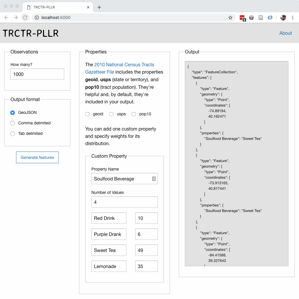
It’s a pleasure following Adrian Miller, a.k.a. @soulfoodscholar, on Twitter. In particular, I get a kick out of voting in and discussing his occasional polls. I’m choosing one of his earliest, concerning soul food beverages, because even though I would never order it, seeing Grape Crush on the menu is a pretty strong real deal indicator. And his category that contains it? Purple Drank: perfect! Although he only got 89 votes in his poll we’re going to fake many more and populate a map.
This screenshot demonstrates how you’d generate a sample of 1000 votes that match @soulfoodscholar’s final distribution.
Popping the resulting GeoJSON into a super-simple Leaflet map looks like this in a screengrab
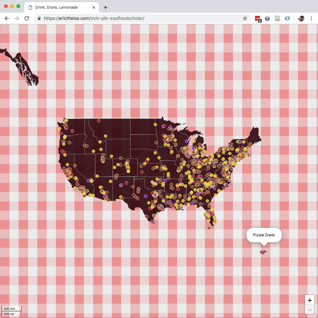
and there’s also an interactive version available.
The Rub
While I am partial to crushing rosemary, sage, fennel seed, and garlic with mortar and pestle this section addresses portability. This project stalled because at the time it didn’t seem I could distribute a large database dump via GitHub. It also didn’t seem reasonable to expect a casual cartographer to set up PostgreSQL with PostGIS, then massage the Census files. I recently learned that GitHub releases can incorporate large files that aren’t under source control in the repository so I’m going to cut and promote a release.
Naming the Application
This application started with a dull-as-dishwater name that I can’t recall. As the logic came into focus it became clear that it was about pulling tracts, which tied it to the motorsport known as tractor pulling in my mind.

But what would be the proper spelling? Tracter seemed more in line with what was going on than tractor but that spelling could easily lead to confusion and well-meaning correctives. The tried and true Internet operation of vowel extraction got me to trctr, and from there I tumbled down to trctr-pllr, a construction nearly identical to that arrived at by Lifter Puller, a mid-1990s band whose sound critic Robert Christgau described as
postpunk noir at the economic margins, drugs and sex and rock and roll in that order, an epic best intoned in toto around a verboten communal ashtray in some after-hours den.
and I’d been listening to Lou Reed take down Christgau in a live recording of Walk on the Wild Side while I was coding.
Perhaps one day I will write about my admiration for LFTR-PLLR and subsequent projects of their frontman and lyricist, Craig Finn.
Caveats
Books, dissertations, whole careers have been devoted to the authority and power of maps. This tool makes it simple to inject quantities of plausible location data into a map or spatial database to help you make decisions about styling, especially dynamic styling, when all you know about your underlying population is that they reside in the United States. It works at the level of the Census Tract. It knows nothing of property parcels, transportation networks, points of interest, or correlations that almost certainly exist between location and the properties you’d ultimately like to render.
Appreciations
Thanks to those who’ve fiddled with TRCTR-PLLR. Special thanks to Éric Lemoine for guiding me through a subtlety of GeoAlchemy2 and Richard Law for the tip on ST_GeneratePoints which I’ve yet to implement although I have created an issue for it.